1. Datasets for Classification
DATA1: Washington DC MALL
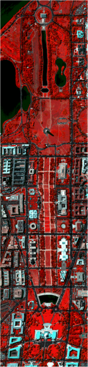
Falsecolor Image
|
|
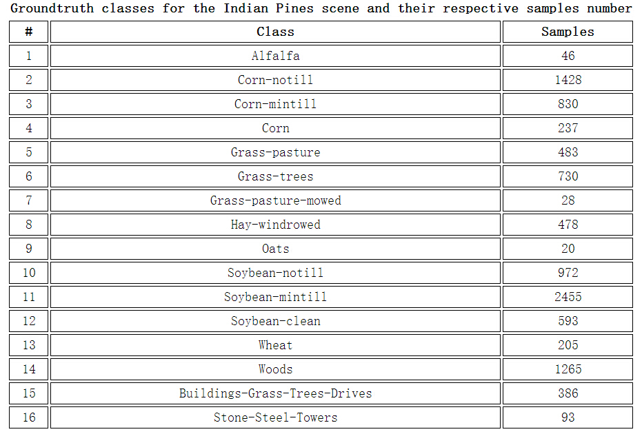
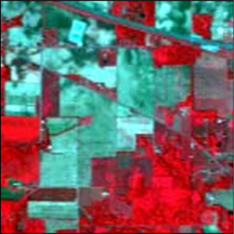
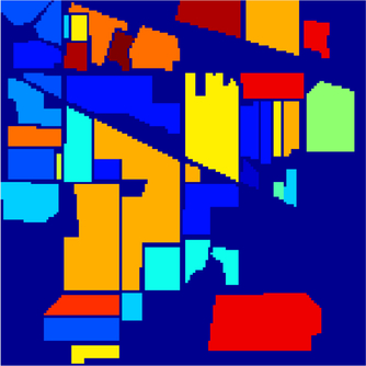
DATA2. Indian Pines
This scene was gathered by AVIRIS sensor over the Indian Pines test site in North-western Indiana and consists of 145\times145 pixels and 224 spectral reflectance bands in the wavelength range 0.4–2.5 10^(-6) meters. This scene is a subset of a larger one. The Indian Pines scene contains two-thirds agriculture, and one-third forest or other natural perennial vegetation. There are two major dual lane highways, a rail line, as well as some low density housing, other built structures, and smaller roads. Since the scene is taken in June some of the crops present, corn, soybeans, are in early stages of growth with less than 5% coverage. The ground truth available is designated into sixteen classes and is not all mutually exclusive. We have also reduced the number of bands to 200 by removing bands covering the region of water absorption: [104-108], [150-163], 220. Indian Pines data are available through Pursue's univeristy MultiSpec site.
Download MATLAB data files: Indian Pines (6.0 MB) | corrected Indian Pines (5.7 MB) | Indian Pines groundtruth (1.1 KB)
|
|
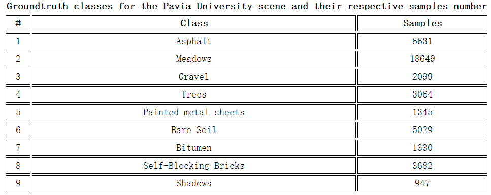
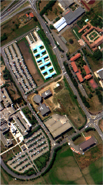
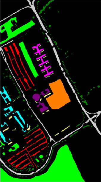
DATA3: University of Pavia
These is the scene acquired by the ROSIS sensor during a flight campaign over Pavia, nothern Italy. The number of spectral bands is 103 for Pavia University. Pavia University is 610*610 pixels, but some of the samples in the images contain no information and have to be discarded before the analysis. The geometric resolution is 1.3 meters. Image groundtruths differenciate 9 classes each. It can be seen the discarded samples in the figures as abroad black strips.
Pavia scenes were provided by Prof. Paolo Gamba from the Telecommunications and Remote Sensing Laboratory, Pavia university (Italy).
Download MATLAB data files: Pavia University (33.2 MB) | Pavia University groundtruth (10.7 KB)
|
|
2. Datasets for Unmixing
It needs to be mentioned that all these datasets are from this website: http://www.escience.cn/people/feiyunZHU/Dataset_GT.html
Note that: These datasets & ground truths are free for research and education only. Please cite our paper listed in BibTex if you use any part of our source code or data.
Note that: These datasets & ground truths are free for research and education only. Please cite our paper listed in BibTex if you use any part of our source code or data.
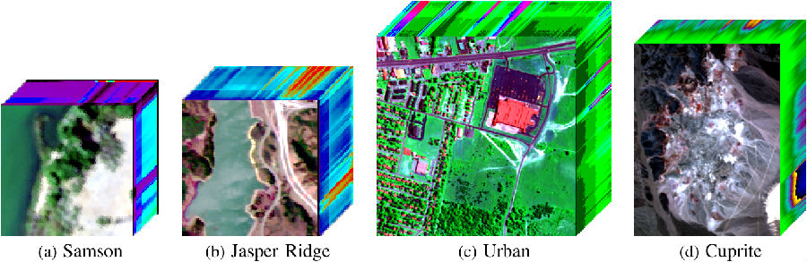
Figure 1. Four real hyperspectral images, i.e. Samson, Jasper Ridge, Urban and Cuprite.
Fig. 1 shows four real hyperspectral images. We give the real dataset in the format of ".img" (Envi) and ".mat" (Matlab). Besides, we provide the corresponding ground truths, which are achieved via the method provided in [SenJia1, SenJia2,SS-NMF]. Please cite our papers summarized in BibTex if you use any part of our source code or data in your research.
#1: Samson (if helpful, please cite the related paper in BibTex)Samson is a simple dataset that is available from the website. In this image, there are 952x 952 pixels. Each pixel is recorded at 156 channels covering the wavelengths from 401 nm to 889 nm. The spectral resolution is highly up to 3.13 nm. As the original image is too large, which is very expensive in terms of computational cost, a region of 95 x 95 pixels is used. It starts from the (252,332)-th pixel in the original image. This data is not degraded by the blank channel or badly noised channels. Specifically, there are three targets in this image, i.e. "#1 Soil", "#2 Tree" and "#3 Water" respectively.
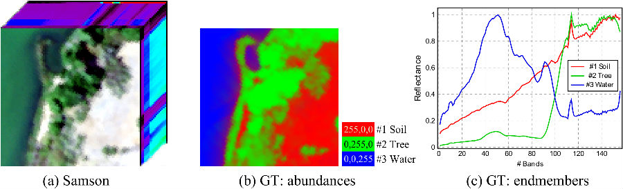
Figure 2. Samson and its ground truths (GT:abundances and GT:endmembers).
Dataset:
#2: Japser Ridge (if helpful, please cite the related paper in BibTex)Jasper Ridge is a popular hyperspectral data used in [enviTutorials, SS-NMF, DgS-NMF,RRLbS, L1-CENMF]. There are 512 x 614 pixels in it. Each pixel is recorded at 224 channels ranging from 380 nm to 2500 nm. The spectral resolution is up to 9.46nm. Since this hyperspectral image is too complex to get the ground truth, we consider a subimage of 100 x 100 pixels. The first pixel starts from the (105,269)-th pixel in the original image. After removing the channels 1--3, 108--112, 154--166 and 220--224 (due to dense water vapor and atmospheric effects), we remain 198 channels (this is a common preprocess for HU analyses). There are four endmembers latent in this data: "#1 Road", "#2 Soil", "#3 Water" and "#4 Tree".
Dataset:
- Data in the Envi format with 156 channels: Data_Envi.zip (1.47Mb)
- Data in the Matlab format with 156 channels: Data_Matlab.zip (3.41Mb)
#2: Japser Ridge (if helpful, please cite the related paper in BibTex)Jasper Ridge is a popular hyperspectral data used in [enviTutorials, SS-NMF, DgS-NMF,RRLbS, L1-CENMF]. There are 512 x 614 pixels in it. Each pixel is recorded at 224 channels ranging from 380 nm to 2500 nm. The spectral resolution is up to 9.46nm. Since this hyperspectral image is too complex to get the ground truth, we consider a subimage of 100 x 100 pixels. The first pixel starts from the (105,269)-th pixel in the original image. After removing the channels 1--3, 108--112, 154--166 and 220--224 (due to dense water vapor and atmospheric effects), we remain 198 channels (this is a common preprocess for HU analyses). There are four endmembers latent in this data: "#1 Road", "#2 Soil", "#3 Water" and "#4 Tree".
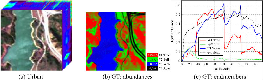
Figure 3. Jasper Ridge and its ground truth (GT:abundances and GT:endmembers).
Dataset:
#3: Urban (if helpful, please cite the related paper in BibTex)
Urban is one of the most widely used hyperspectral data used in the hyperspectral unmixing study. There are 307 x 307 pixels, each of which corresponds to a 2 x 2 m2area. In this image, there are 210 wavelengths ranging from 400 nm to 2500 nm, resulting in a spectral resolution of 10 nm. After the channels 1--4, 76, 87, 101--111, 136--153 and 198--210 are removed (due to dense water vapor and atmospheric effects), we remain 162 channels (this is a common preprocess for hyperspectral unmixing analyses). There are three versions of ground truth, which contain 4, 5 and 6 endmembers respectively, which are introduced in the ground truth.
Dataset:
- Data in the Envi format with 198 channels: jasperRidge2_R198.zip (2.87Mb)
- Data in the Envi format with 224 channels: jasperRidge2_F224.zip (2.98Mb)
- Data in the Matlab format with 198 channels: jasperRidge2_R198.mat (2.84Mb)
- Data in the Matlab format with 224 channels: jasperRidge2_F224.mat (3.01Mb)
#3: Urban (if helpful, please cite the related paper in BibTex)
Urban is one of the most widely used hyperspectral data used in the hyperspectral unmixing study. There are 307 x 307 pixels, each of which corresponds to a 2 x 2 m2area. In this image, there are 210 wavelengths ranging from 400 nm to 2500 nm, resulting in a spectral resolution of 10 nm. After the channels 1--4, 76, 87, 101--111, 136--153 and 198--210 are removed (due to dense water vapor and atmospheric effects), we remain 162 channels (this is a common preprocess for hyperspectral unmixing analyses). There are three versions of ground truth, which contain 4, 5 and 6 endmembers respectively, which are introduced in the ground truth.
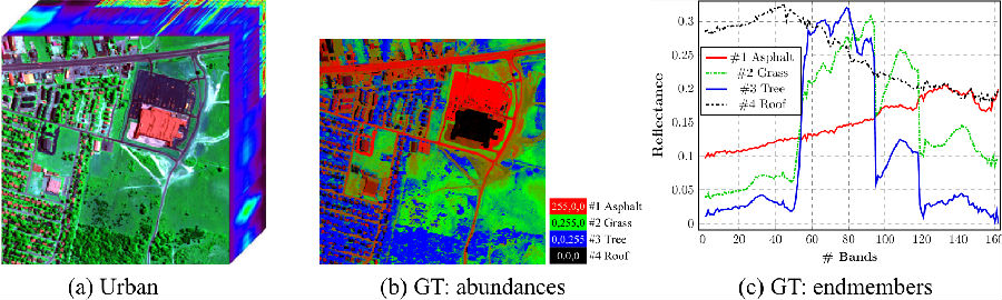
Figure 4. Urban and its ground truths (4 endmember version).
Dataset:
#4: Cuprite (if helpful, please cite the related paper in BibTex)
Cuprite (available form website) is the most benchmark dataset for the hyperspectral unmixing research that covers the Cuprite in Las Vegas, NV, U.S. There are 224 channels, ranging from 370 nm to 2480 nm. After removing the noisy channels (1--2 and 221--224) and water absorption channels (104–113 and 148–167), we remain 188 channels. Aregion of 250 x 190 pixels is considered, where there are 14 types of minerals. Since there are minor differences between variants of similar minerals, we reduce the number of endmembers to 12, which are summarized as follows "#1 Alunite", "#2 Andradite", "#3 Buddingtonite", "#4 Dumortierite", "#5 Kaolinite1", "#6 Kaolinite2", "#7 Muscovite", "#8 Montmorillonite", "#9 Nontronite", "#10 Pyrope", "#11 Sphene", "#12 Chalcedony".
Dataset:
- Data in the Envi format with 221 channels: Urban_F210.zip (19.5Mb)
- Data in the Matlab format with 162 channels: Urban_R162.mat (16.9Mb)
- Data in the Matlab format with 221 channels: Urban_F210.mat (21.8Mb)
- 4 endmembers version: GroundTruth (3.7Mb). The 4 endmembers are "#1 Asphalt", "#2 Grass", "#3 Tree" and "#4 Roof" respectively.
- 5 endmembers version: GroundTruth (3.65Mb). The 5 endmembers are "#1 Asphalt", "#2 Grass", "#3 Tree", "#4 Roof" and "#5 Dirt" respectively.
- 6 endmembers version: GroundTruth (3.92Mb). The 6 endmembers are "#1 Asphalt", "#2 Grass", "#3 Tree", "#4 Roof", "#5 Metal", and "6 Dirt" respectively.
#4: Cuprite (if helpful, please cite the related paper in BibTex)
Cuprite (available form website) is the most benchmark dataset for the hyperspectral unmixing research that covers the Cuprite in Las Vegas, NV, U.S. There are 224 channels, ranging from 370 nm to 2480 nm. After removing the noisy channels (1--2 and 221--224) and water absorption channels (104–113 and 148–167), we remain 188 channels. Aregion of 250 x 190 pixels is considered, where there are 14 types of minerals. Since there are minor differences between variants of similar minerals, we reduce the number of endmembers to 12, which are summarized as follows "#1 Alunite", "#2 Andradite", "#3 Buddingtonite", "#4 Dumortierite", "#5 Kaolinite1", "#6 Kaolinite2", "#7 Muscovite", "#8 Montmorillonite", "#9 Nontronite", "#10 Pyrope", "#11 Sphene", "#12 Chalcedony".
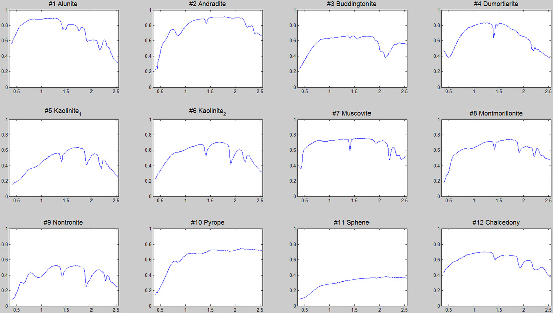
Figure 5. The ground truth for Cuprite (12 endmembers).
Dataset:
Dataset:
- Data in the Envi format with 224 channels: Cuprite_S1_F224.zip (14.0Mb)
- Data in the Envi format with 188 channels: Cuprite_S1_R188.zip (12.9Mb)
- Data in the Matlab format with 224 channels: Cuprite_S1_F224.mat (15.4Mb)
- Data in the Matlab format with 188 channels: Cuprite_S1_R188.mat (13.7Mb)
3. HSI SYNTHESIS TOOLS for MATLAB (for Unmixing)
It needs to be mentioned that all these datasets are from the website:
http://www.ehu.eus/ccwintco/index.php?title=Hyperspectral_Imagery_Synthesis_tools_for_MATLAB
http://www.ehu.eus/ccwintco/index.php?title=Hyperspectral_Imagery_Synthesis_tools_for_MATLAB
Download the latest Hyperspectral Imagery Synthesis toolbox for MATLAB here:
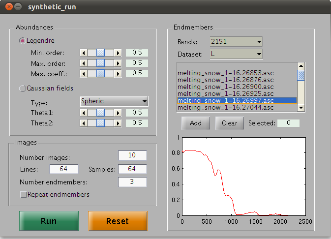
This software is distributed under the terms of the GNU General Public License as published by the Free Software Foundation, either version 3 of the License, or (at your option) any later version. The Synthesis tools package has been actually developed with MATLAB 7.4 software (http://www.mathworks.com/) and a licensed copy is needed to use it.
If you are using the Hyperspectral Imagery Synthesis toolbox for your scientific research, please reference it as follows:
Hyperspectral Imagery Synthesis (EIAs) toolbox.
Grupo de Inteligencia Computacional, Universidad del País Vasco / Euskal Herriko Unibertsitatea (UPV/EHU), Spain. http://www.ehu.es/ccwintco/index.php/Hyperspectral_Imagery_Synthesis_tools_for_MATLAB
Copyright 2010 Grupo Inteligencia Computacional, Universidad del País Vasco / Euskal Herriko Unibertsitatea (UPV/EHU).
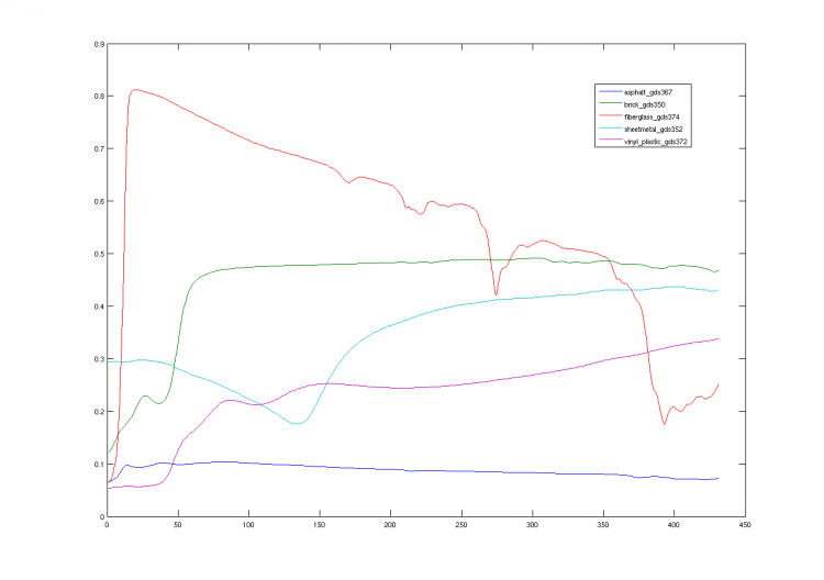
IC Synthetic Hyperspectral CollectionHere you can find a set of hyperspectral synthetic images generated by the "Synthesis tools" package. All these synthetic images have been generated using five selected endmembers from the USGS spectral library included in the "Synthesis tools" package (see figure above). Each image's spatial dimensions are of 128x128 pixels and they have 431 spectral bands. The hyperspectral synthetic image collections are distributed in ZIP files containing five MAT files each. One of this MAT files corresponds to the free of noise hyperspectral synthetic image, and in the other four additive noise has been added to the synthetic image given a Signal to Noise Ratio (SNR) of 20, 40, 60 and 80db respectively.
If you are using the Hyperspectral Imagery Synthesis toolbox for your scientific research, please reference it as follows:
Hyperspectral Imagery Synthesis (EIAs) toolbox.
Grupo de Inteligencia Computacional, Universidad del País Vasco / Euskal Herriko Unibertsitatea (UPV/EHU), Spain. http://www.ehu.es/ccwintco/index.php/Hyperspectral_Imagery_Synthesis_tools_for_MATLAB
Copyright 2010 Grupo Inteligencia Computacional, Universidad del País Vasco / Euskal Herriko Unibertsitatea (UPV/EHU).
IC Synthetic Hyperspectral CollectionHere you can find a set of hyperspectral synthetic images generated by the "Synthesis tools" package. All these synthetic images have been generated using five selected endmembers from the USGS spectral library included in the "Synthesis tools" package (see figure above). Each image's spatial dimensions are of 128x128 pixels and they have 431 spectral bands. The hyperspectral synthetic image collections are distributed in ZIP files containing five MAT files each. One of this MAT files corresponds to the free of noise hyperspectral synthetic image, and in the other four additive noise has been added to the synthetic image given a Signal to Noise Ratio (SNR) of 20, 40, 60 and 80db respectively.
The IC Synthetic Hyperspectral Collections:
- Legendre: download (247.4 Mb)
- Spheric Gaussian Field: download (255.0 Mb)
- Exponential Gaussian Field: download (256.2 Mb)
- Rational Gaussian Field: download (256.5 Mb)
- Matern Gaussian Field: download (255.2 Mb)
